What The Curve


x = 0.01:0.01:20;
y = x .^ (-log(x));
y1 = y;
for i = 1:numel(y)
y1(i) = trapz(y(1:i));
end
y1 = y1/max(y1);
plot(x,y1, x,y);
print -dpng figure.png


Speed of Light © 2.99792458e+8 m*s-1
Planck constant (h) 6.626068963e-34 J*s
Boltzmann constant (k) 1.3806504e-23 J*K-1
Wien constant (b) 2.8977685e-3 m*K
Stefan-Boltzmann constant (σ) 5.670400e-8 W*m-2*K-4
First Radiation constant for spectral radiance (c1) (2hc2) 1.191042759e-16 W*m2*sr-1
Second Radiation constant (c2) (hc/k) 1.4387752e-2 m*K

h = 6.63E-34 Js
c = 299792458 m/s
k = 1.38E-23 J/K
e = 2.71828
z = 4.9651142
b = 2.89777E-03 mK
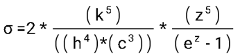
σ = 2k5z5/h4c3(e^z) = 4.06711E-06
L_λmax(T) = σ*T⁵
λmax(T) = (b/T)
pow(λ/λmax(T), -2*ln(λ/λmax(T))*L_λmax(T)


Planck = hf * 2c/x4/(exp(hc/kxt)-1)


Ch/ktx = a


x_max(t) = ch/kta
L_max(t) = t4*2*(k4a4/h4c3) / (e^(1/a)-1)
F(X) = 2c/x4/(e^(hc/ktx)-1)
= F(X*x_max)/L_max

F’(x) = 1/x⁴ * (e^(1/a)-1)/( e^(1/ax)-1)
Maxwell-Boltzmann distribution

Maxwell-Boltzmann distribution birim fonksiyonu


G Force


https://www.tutorialspoint.com/execute_matlab_online.php
offset = 0.25;
sample = 1000;
dt = (pi-offset)/sample;
theta = (offset:dt:pi) — offset / 2;
x0 = 0:0.01:5; % x position of moving referance point
p = exp(i*[theta theta+pi]);
scatter(real(p), imag(p));
daspect([1 1 1]);
print -dpng figure2.png
p0 = x0; % moving referance point
r = p’-p0; % distance vector
r_unit = r./abs(r); % unit vector of distace vector
g = (1./abs(r) .^ 2); % scalar G force
f = r_unit .* g; % force vector
figure;
plot(x0, abs(sum(f*dt)));
title(‘Gravity Force Curve’);
xlabel(‘Distance’);
ylabel(‘Force’);
print -dpng figure.png


offset = 1.00;


offset = 2;
sample = 50;
dt = (pi-offset)/sample;theta = (offset:dt:pi) — offset / 2;
x0 = 0:0.01:5; % x position of moving referance pointp = exp(i*[theta theta+pi]); % circle
p = [];
for dr = 0.18:0.01:1
l = 2*sqrt(1-dr*dr);
dt = 2/((l+1/sample)*sample);
p1 = (-1:dt:1)*l/2; p = [p p1+dr*i p1-dr*i]; % straight
end
disp(‘number of sample:’);
disp(numel(p));scatter(real(p), imag(p));
daspect([1 1 1]);
print -dpng figure2.pngp0 = x0; % moving referance point
r = p’-p0; % distance vectorr_unit = r./abs(r); % unit vector of distace vector
g = (1./abs(r) .^ 2); % scalar G force
f = r_unit .* g; % force vector
figure;
Fx0 = abs(sum(f)/numel(p));
plot(x0, Fx0);
daspect([1 1 1]);disp(Fx0((x0 > 2.9) & (x0 < 3.1)));
title(‘Gravity Force Curve’);
xlabel(‘Distance’);
ylabel(‘Force’);
print -dpng figure.pngfigure;
iFx0 = cumtrapz(x0, Fx0);
plot(x0, iFx0);
daspect([1 1 1]);
print -dpng figure.png


N(r) =M(r)/dm
M_3(r) = 4*pi*r²
dx = s*F*dr
cos(t) = dr/(dr+dxs)
dxs = s*Fs*dr = (1/cos(t) -1)dr
k = 1/(s*dr)
Fs = dxs*k
F0 = N(r)*Fs*sin(t) = dx0 * k
F0 = N(r)/s * (1/cos(t) -1)*sin(t)
s*F0/N(r) = tan(t) -sin(t)
s*F0*dm/(4*pi*r²) = tan(t) -sin(t)
r = sqrt(s*F0*dm/(4*pi*(tan(t) -sin(t))))
s*F0*dm/(4*pi*) = 1 => r = sqrt(1/(tan(t) -sin(t)))
cos(t) = density
tan(t) = dy
https://www.desmos.com/calculator
\left(\left(\tan\left(t\right)-\sin\left(t\right)\right)^{-\frac{1}{2}},\cos\left(t\right)\right)
\left(\left(\tan\left(t\right)-\sin\left(t\right)\right)^{-\frac{1}{2}},\ -\frac{\sin\left(t\right)}{-\frac{\left(\left(\sec\left(t\right)\right)^{2}-\cos\left(t\right)\right)}{2\cdot\left(\tan\left(t\right)-\sin\left(t\right)\right)^{\frac{3}{2}}}}\right)


Divide[\(40)D[Divide[sin\(40)t\(41),\(40)Divide[\(40)Power[sec\(40)t\(41),2]-cos\(40)t\(41)\(41),\(40)2*Power[\(40)tan\(40)t\(41)-sin\(40)t\(41)\(41),\(40)Divide[3,2]\(41)]\(41)]\(41)],t]\(41),D[Power[\(40)tan\(40)t\(41)-sin\(40)t\(41)\(41),\(40)Divide[-1,2]\(41)],t]]=0

t = 1.354771 => y’’ = 0
https://www.desmos.com/calculator
\left(\frac{\left(\tan\left(t\right)-\sin\left(t\right)\right)^{-\frac{1}{2}}}{0.528509317863},\ \frac{\frac{\sin\left(t\right)}{\left(\frac{\left(\left(\sec\left(t\right)\right)^{2}-\cos\left(t\right)\right)}{2\cdot\left(\tan\left(t\right)-\sin\left(t\right)\right)^{\frac{3}{2}}}\right)}}{0.614044725811}\right)

OMG!